Jump Markov chains and rejection-free Metropolis algorithms

In this section, we introduce applications and simulations to illustrate the advantage of Rejection-Free algorithm. We compare the efficiency of the Rejection-Free and standard Metropolis algorithms in three different examples. The first example is a Bayesian inference model on a real data set taken from the Education Longitudinal Study of National Center (2002). The second example involves sampling from a two-dimensional ferromagnetic $4 \times 4$ Ising model. The third example is a pseudo-marginal Andrieu and Roberts (2009) version of the Ising model. All three simulations show that the introduction of the Rejection-Free method leads to significant speedup. This provides concrete numerical evidence for the efficiency of using the rejection-free approach to improve the convergence to stationarity of the algorithms.

A Bayesian inference problem with real data

For our first example, we consider the Education Longitudinal Study data from the National Center (2002), a real data set consisting of final course grades of over 9000 students. We take a random subset of 200 of these 9000 students, and denote their scores as $x_1, x_2, \dots , x_{200}$. (Note that all scores in this data set are integers between 0 and 100.)

Our parameter of interest $\theta $ is the true average value of the final grades for these 200 students, rounded to 1 decimal place (so $\theta \in \{0.1, 0.2, 0.3, \dots , 99.7, 99.8, 99.9\}$ is still discrete, and can be studied using specialised computer hardware). The likelihood function for this model is the binomial distribution

$$\begin{aligned} \mathbf{L }(x|\theta ) = {100 \atopwithdelims ()x} \, \theta ^x \, (1-\theta )^{100-x} \, . \end{aligned}$$

(13)

For our prior distribution, we take

$$\begin{aligned} \theta \ \sim \ \text {Uniform}\{0.1, 0.2, 0.3, \dots , 99.7, 99.8, 99.9\} \, . \end{aligned}$$

(14)

The posterior distribution $\pi (\theta )$ is then proportional to the prior probability function (14) times the likelihood function (13).

We ran an Independence Sampler for this posterior distribution, with fixed proposal distribution equal to the prior (14), either with or without the Rejection-Free modification. For each of these two algorithms, we calculated the effective sample size, defined as

$$\begin{aligned} \textit{ESS}(\theta ) = \frac{N}{1+ 2 \sum _{k=1}^\infty \rho _k(\theta )} \, , \end{aligned}$$

where N is the number of posterior samples, and $\rho _k(\theta )$ represents autocorrelation at lag k for the posterior samples of $\theta $. (For a chain of finite length, the sum $\sum _{k=1}^\infty \rho _k(\theta )$ cannot be taken over all k, so instead we just sum until the values of $\rho _k(\theta )$ become negligible.) For fair comparison, we consider both the ESS per iteration, and the ESS per second of CPU time.

Table 1 Median effective sample size from 100 runs of each of the metropolis and rejection-free algorithms, for the Bayesian real data example of Sect. 7.1

Full size table

Table 1 presents the median ESS per iteration, and median ESS per second, from 100 runs of 100,000 iterations each, for each of the two algorithms. We see from Table 1 that Rejection-Free outperforms the Metropolis algorithm by a factor of about 75 or 64, in terms of ESS per iteration or ESS per second. This clearly illustrates the efficiency of the Rejection-Free algorithm.

An expanded real data example

In the previous example, we consider a random subset of 200 students from the National Center (2002) data set. We now consider data from all 9000 students simultaneously.

In this case, with so many data, the posterior will tend to be quite concentrated, in this case around the value 51.1. Hence, the old prior is not suitable anymore. Instead, we need to keep accuracy to at least 2 decimals to get a well-distributed posterior. Therefore, we instead choose the prior $\theta \sim \text {Uniform}\{0.01, 0.02, 0.03, \ldots , 99.97, 99.98, 99.99\}$, to be accurate to two decimal places.

We ran each of the two algorithms for 100 runs of 100,000 iterations each, using all the data from the dataset. Table 4 presents the resulting median ESS per iteration, and median ESS per second.

Table 2 Median effective sample size from 100 runs of each of the metropolis and rejection-free algorithms, for the expanded Bayesian real data example of Sect. 7.2

Full size table

We see from Table 4 that Rejection-Free again outperforms the Metropolis algorithm, this time by factors of over 40. This again illustrates the efficiency of the Rejection-Free algorithm, even for very large real datasets.

Simulations of an Ising model

We next present a simulation study of a ferromagnetic Ising model on a two-dimensional $4 \times 4$ square latice. The energy function for this model is given by

$$\begin{aligned} E(S) = - \sum _{i

where each spin $s_i,s_j \in \{-1,1\}$, and $J_{i j}$ represents the interaction between the $i^\mathrm{th}$ and $j^\mathrm{th}$ spins. To make only the neighbouring spins in the lattice interact with each other, we take $J_{i j} = 1$ for all neighbours i and j, and $J_{i j}$ = 0 otherwise. The Ising model then has probability distribution propositional to the exponential of the energy function:

$$\begin{aligned} \Pi (S) \ \propto \ \exp [-E(S)] \, . \end{aligned}$$

We investigate the efficiency of the samples produced in four different scenarios: Metropolis algorithm and Rejection-Free, both with and without Parallel Tempering. For the Parallel Tempering versions, we set

$$\begin{aligned} \Pi _T(S) \ \propto \ \exp [-E(S) \, / \, T] \, . \end{aligned}$$

Here $T = 1$ is the temperature of interest (which we want to sample from). We take $T = 2$ as the highest temperature, since when $T = 2$ the probability distribution for magnetization is quite flat (with highest probability $\mathbf{P }[M(S) = 14] = 0.083$, and lowest probability $\mathbf{P }[M(S) = 2] = 0.037$). Including the one additional temperature $T = \sqrt{2}$ gives three temperatures $1, \sqrt{2}, 2$ in geometric progression, with average swap acceptance rate $31.6\%$ which is already higher than the $23.4\%$ recommended in Roberts and Rosenthal (2014), indicating that three temperatures is enough.

We study convergence of the magnetization value, where the magnetization of a given state S of the Ising model is defined as:

$$\begin{aligned} M(S) = \sum _i s_i. \end{aligned}$$

For our $4 \times 4$ Ising model,

$$\begin{aligned} M(S) \in {\mathcal {M}} = \{-16, -14, -12, \dots , -2, 0, 2, \dots , 12, 14, 16\}. \end{aligned}$$

We measure the distance to stationarity by the total variation distance between the sampled and the actual magnetization distributions after n iterations, defined as:

$$\begin{aligned} \text {TVD}(n) = \frac{1}{2} \sum _{m \in {\mathcal {M}}} \Big | \mathbf{P}[M(X_n)=m] - \Pi \{S : M(S)=m\} \Big | \, , \end{aligned}$$

where $M(X_n)$ is the magnetization of the chain at iteration n, and $\Pi \{S : M(S)=m\}$ represents the stationary probability of magnetization value m. Thus, convergence to stationarity is described by how quickly TVD(n) decreases to 0.

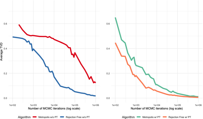
Figure 8 lists the average total variation distance TVD(n) for each version, as a function of the number of iterations n, based on 100 runs of each of the four scenarios, of $10^6$ iterations each. It illustrates that, with or without Parallel Tempering, the use of Rejection-Free provides significant speedup, and TVD decreases much more rapidly with the Rejection-Free method than without it. This provides concrete numerical evidence for the efficiency of using Rejection-Free to improve the convergence to stationarity of the algorithm.

We next consider the issue of computational cost. The Rejection-Free method requires computing probabilities for all neighbors of the current state. However, with specialised computer hardware, Rejection-Free can be very efficient since the calculation of the probabilities for all neighbours and selection of the next state can both be done in parallel. The computational cost of each iteration of Rejection-Free is therefore equal to the maximum cost used on each neighbor. Similarly, for Parallel Tempering, we can calculate all of the different temperature chains in parallel. The average CPU time per iteration for each of the four different scenarios are presented in Table 3. It illustrates that the computational cost of Rejection-Free without Parallel Tempering was comparable to that of the usual Metropolis algorithm, though Rejection-Free with Parallel Tempering does require up to 50% more time than the other three scenarios.

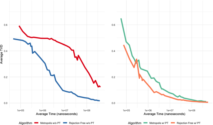
Table 3 Average CPU time per iteration for the Ising Model example of Sect. 7.3, for each of four scenarios:

Full size table

Figure 9 shows the average total variation distance as a function of the total CPU time used for each algorithm. Figure 9 is quite similar to Fig. 8, and gives the same overall conclusion: with or without Parallel Tempering, the use of Rejection-Free provides significant speedup, even when computational cost is taken into account.

As a final check, we also calculated the effective sample size, similar to the first example. First, we generated 100 MCMC chains of 100,000 iterations each, from all four algorithms. Then, we calculated the effective sample size for each chain, and normalized the results by either the number of iterations or the total CPU time for each algorithm. Table 4 shows the median of ESS per iteration and ESS per CPU second. It again illustrates that Rejection-Free can produce great speedups, increasing the ESS per CPU second by a factor of over 50 without Parallel Tempering, or a factor of 2 with Parallel Tempering.

Table 4 Median of normalized effective sample sizes for the Ising model example of Sect. 7.3, for four scenarios: Metropolis and Rejection-Free, both with and without Parallel Tempering

Full size table

A pseudo-marginal MCMC example

If the target density itself is not available analytically, but an unbiased estimate exists, then pseudo-marginal MCMC Andrieu and Roberts (2009) can still be used to sample from the correct target distribution. We next apply the Rejection-Free method to a pseudo-marginal algorithm to show that Rejection-Free can provide speedups in that case, too.

In the previous example of the $4 \times 4$ Ising model, the target probability distributions were defined as

$$\begin{aligned} \Pi (S) \ \propto \ \exp \left\{ - \frac{E(S)}{T}\right\} \, . \end{aligned}$$

We now pretend that this target density is not available, and we only have access to an unbiased estimator given by

$$\begin{aligned} \Pi _0(S) \ \propto \ \Pi (S) \times A = \exp \left\{ \frac{E(S)}{T}\right\} \times A \, , \end{aligned}$$

where $A \sim \text {Gamma}(\alpha = 10, \beta = 10)$ is a random variable (which is sampled independently every time as we try to compute the target distribution). Note that $\mathbf{E}(A) = 10/10 = 1$, so $\mathbf{E}[\Pi _0(S)] = \Pi (S)$, and the estimator is unbiased (though A has variance $10/10^2 = 1/10 > 0$).

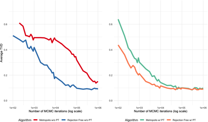
Using this unbiased estimate of the target distribution as for pseudo-marginal MCMC, we again investigated the convergence of samples produced by the same four scenarios: Metropolis and Rejection-Free, both with and without Parallel Tempering. Figure 10 shows the average total variation distance TVD(n) between the sampled and the actual magnetization distributions, for 100 chains, as a function of the iteration n, keeping all the other settings the same as before. This figure is quite similar to Fig. 8, again showing that with or without Parallel Tempering, the use of Rejection-Free provides significant speedup, even in the pseudo-marginal case.